PINNs Burger’s equation#
The one dimensional Burger’s equation is given by: $\(\frac{\partial u}{\partial t} + u \frac{\partial u}{\partial x} = \nu \frac{\partial^2 u}{\partial x^2}; \;\;\; x \in [-1, 1], t \in [0,1]\)$
This equation can be solved numerically with appropriate initial and boundary conditions. In this notebook, a physics informed neural network is trained to learn the solution of the Burger’s equation.
Import necessary tools#
In the following cell we import the necessary libraries to set up the environment to run the code.
!pip3 install torch==2.1.0 torchvision==0.16.0 torchaudio==2.1.0 --index-url https://download.pytorch.org/whl/cpu
Defaulting to user installation because normal site-packages is not writeable
Looking in indexes: https://download.pytorch.org/whl/cpu
Collecting torch==2.1.0
  Downloading https://download.pytorch.org/whl/cpu/torch-2.1.0%2Bcpu-cp311-cp311-linux_x86_64.whl (184.9 MB)
     ━━━━━━━━━━━━━━━━━━━━━━━━━━━━━━━━━━━━━━ 184.9/184.9 MB 29.9 MB/s eta 0:00:0000:0100:01
?25hCollecting torchvision==0.16.0
  Downloading https://download.pytorch.org/whl/cpu/torchvision-0.16.0%2Bcpu-cp311-cp311-linux_x86_64.whl (1.6 MB)
     ━━━━━━━━━━━━━━━━━━━━━━━━━━━━━━━━━━━━━━━━ 1.6/1.6 MB 6.4 MB/s eta 0:00:0000:0100:01
?25hCollecting torchaudio==2.1.0
  Downloading https://download.pytorch.org/whl/cpu/torchaudio-2.1.0%2Bcpu-cp311-cp311-linux_x86_64.whl (1.6 MB)
     ━━━━━━━━━━━━━━━━━━━━━━━━━━━━━━━━━━━━━━━━ 1.6/1.6 MB 7.6 MB/s eta 0:00:0000:0100:01
?25hCollecting filelock (from torch==2.1.0)
  Downloading https://download.pytorch.org/whl/filelock-3.13.1-py3-none-any.whl (11 kB)
Requirement already satisfied: typing-extensions in /opt/conda/lib/python3.11/site-packages (from torch==2.1.0) (4.8.0)
Collecting sympy (from torch==2.1.0)
  Downloading https://download.pytorch.org/whl/sympy-1.12-py3-none-any.whl (5.7 MB)
     ━━━━━━━━━━━━━━━━━━━━━━━━━━━━━━━━━━━━━━━━ 5.7/5.7 MB 31.4 MB/s eta 0:00:00:00:0100:01
?25hCollecting networkx (from torch==2.1.0)
  Downloading https://download.pytorch.org/whl/networkx-3.2.1-py3-none-any.whl (1.6 MB)
     ━━━━━━━━━━━━━━━━━━━━━━━━━━━━━━━━━━━━━━━━ 1.6/1.6 MB 10.4 MB/s eta 0:00:00:00:01
?25hRequirement already satisfied: jinja2 in /opt/conda/lib/python3.11/site-packages (from torch==2.1.0) (3.1.2)
Collecting fsspec (from torch==2.1.0)
  Downloading https://download.pytorch.org/whl/fsspec-2024.2.0-py3-none-any.whl (170 kB)
     ━━━━━━━━━━━━━━━━━━━━━━━━━━━━━━━━━━━━━━━ 170.9/170.9 kB 2.5 MB/s eta 0:00:00a 0:00:01
?25hRequirement already satisfied: numpy in /opt/conda/lib/python3.11/site-packages (from torchvision==0.16.0) (1.26.2)
Requirement already satisfied: requests in /opt/conda/lib/python3.11/site-packages (from torchvision==0.16.0) (2.31.0)
Requirement already satisfied: pillow!=8.3.*,>=5.3.0 in /opt/conda/lib/python3.11/site-packages (from torchvision==0.16.0) (10.1.0)
Requirement already satisfied: MarkupSafe>=2.0 in /opt/conda/lib/python3.11/site-packages (from jinja2->torch==2.1.0) (2.1.3)
Requirement already satisfied: charset-normalizer<4,>=2 in /opt/conda/lib/python3.11/site-packages (from requests->torchvision==0.16.0) (3.3.0)
Requirement already satisfied: idna<4,>=2.5 in /opt/conda/lib/python3.11/site-packages (from requests->torchvision==0.16.0) (3.4)
Requirement already satisfied: urllib3<3,>=1.21.1 in /opt/conda/lib/python3.11/site-packages (from requests->torchvision==0.16.0) (2.0.7)
Requirement already satisfied: certifi>=2017.4.17 in /opt/conda/lib/python3.11/site-packages (from requests->torchvision==0.16.0) (2023.7.22)
Collecting mpmath>=0.19 (from sympy->torch==2.1.0)
  Downloading https://download.pytorch.org/whl/mpmath-1.3.0-py3-none-any.whl (536 kB)
     ━━━━━━━━━━━━━━━━━━━━━━━━━━━━━━━━━━━━━━ 536.2/536.2 kB 22.6 MB/s eta 0:00:00
?25hInstalling collected packages: mpmath, sympy, networkx, fsspec, filelock, torch, torchvision, torchaudio
  WARNING: The script isympy is installed in '/home/tg458981/work/HPCWork/.jupyter-lab-hpc/.local/bin' which is not on PATH.
  Consider adding this directory to PATH or, if you prefer to suppress this warning, use --no-warn-script-location.
  WARNING: The scripts convert-caffe2-to-onnx, convert-onnx-to-caffe2 and torchrun are installed in '/home/tg458981/work/HPCWork/.jupyter-lab-hpc/.local/bin' which is not on PATH.
  Consider adding this directory to PATH or, if you prefer to suppress this warning, use --no-warn-script-location.
Successfully installed filelock-3.13.1 fsspec-2024.2.0 mpmath-1.3.0 networkx-3.2.1 sympy-1.12 torch-2.1.0+cpu torchaudio-2.1.0+cpu torchvision-0.16.0+cpu
!pip3 install matplotlib numpy tqdm scipy pyDOE --user
Requirement already satisfied: matplotlib in /opt/conda/lib/python3.11/site-packages (3.8.2)
Requirement already satisfied: numpy in /opt/conda/lib/python3.11/site-packages (1.26.2)
Requirement already satisfied: tqdm in /opt/conda/lib/python3.11/site-packages (4.66.1)
Collecting scipy
  Downloading scipy-1.14.0-cp311-cp311-manylinux_2_17_x86_64.manylinux2014_x86_64.whl.metadata (60 kB)
     ━━━━━━━━━━━━━━━━━━━━━━━━━━━━━━━━━━━━━━━━ 60.8/60.8 kB 1.1 MB/s eta 0:00:00a 0:00:01
?25hCollecting pyDOE
  Using cached pyDOE-0.3.8.zip (22 kB)
  Preparing metadata (setup.py) ... ?25ldone
?25hRequirement already satisfied: contourpy>=1.0.1 in /opt/conda/lib/python3.11/site-packages (from matplotlib) (1.2.0)
Requirement already satisfied: cycler>=0.10 in /opt/conda/lib/python3.11/site-packages (from matplotlib) (0.12.1)
Requirement already satisfied: fonttools>=4.22.0 in /opt/conda/lib/python3.11/site-packages (from matplotlib) (4.46.0)
Requirement already satisfied: kiwisolver>=1.3.1 in /opt/conda/lib/python3.11/site-packages (from matplotlib) (1.4.5)
Requirement already satisfied: packaging>=20.0 in /opt/conda/lib/python3.11/site-packages (from matplotlib) (23.2)
Requirement already satisfied: pillow>=8 in /opt/conda/lib/python3.11/site-packages (from matplotlib) (10.1.0)
Requirement already satisfied: pyparsing>=2.3.1 in /opt/conda/lib/python3.11/site-packages (from matplotlib) (3.1.1)
Requirement already satisfied: python-dateutil>=2.7 in /opt/conda/lib/python3.11/site-packages (from matplotlib) (2.8.2)
Requirement already satisfied: six>=1.5 in /opt/conda/lib/python3.11/site-packages (from python-dateutil>=2.7->matplotlib) (1.16.0)
Downloading scipy-1.14.0-cp311-cp311-manylinux_2_17_x86_64.manylinux2014_x86_64.whl (41.1 MB)
   ━━━━━━━━━━━━━━━━━━━━━━━━━━━━━━━━━━━━━━━━ 41.1/41.1 MB 47.6 MB/s eta 0:00:00:00:0100:01
?25hBuilding wheels for collected packages: pyDOE
  Building wheel for pyDOE (setup.py) ... ?25ldone
?25h  Created wheel for pyDOE: filename=pyDOE-0.3.8-py3-none-any.whl size=18168 sha256=77c43d8710ca85466cd75b8b669f8d9a30188e33ac407821ee160e6f0a363e53
  Stored in directory: /home/tg458981/work/HPCWork/.jupyter-lab-hpc/.cache/pip/wheels/84/20/8c/8bd43ba42b0b6d39ace1219d6da1576e0dac81b12265c4762e
Successfully built pyDOE
Installing collected packages: scipy, pyDOE
Successfully installed pyDOE-0.3.8 scipy-1.14.0
# Import necessary libraries
import torch
import torch.nn as nn
import numpy as np
import scipy
from scipy import io
from pyDOE import lhs
import time
from scipy.interpolate import griddata
import matplotlib.pyplot as plt
from tqdm import tqdm
Define the neural network#
Once the libraries are loaded, we build the neural networks. We build two neural networks, one (net_u) for predicting the solution \(u\) and the other (net_f) for predicting the residual of the governing equation \(f(u)\). The number of layers and neurons in each layer is taken as a list input to construct the network net_u. The residuals in the network net_f are computed using the derivatives of the solutions computing using automatic differentiation.
# Define a network for predicting u

layers = [2, 20, 20, 20, 20, 20, 20, 20, 20, 1]

layer_list = []
for l in range(len(layers)-1):
    layer_list.append(nn.Linear(layers[l],layers[l+1]))
    layer_list.append(nn.Tanh())


net_u = nn.Sequential(*layer_list)

# Define a network for predicting f

def net_f(x, t, nu):
    x.requires_grad = True
    t.requires_grad = True
    u = net_u(torch.cat([x,t],1))
    u_t = torch.autograd.grad(u, t, create_graph=True, grad_outputs=torch.ones_like(u),
                     allow_unused=True)[0]
    u_x = torch.autograd.grad(u, x, create_graph=True,
                     grad_outputs=torch.ones_like(u),
                     allow_unused=True)[0]
    u_xx = torch.autograd.grad(u_x, x, create_graph=True,
                     grad_outputs=torch.ones_like(u),
                     allow_unused=True)[0]
    f = u_t + u * u_x - nu * u_xx
    return f
Define functions to train and predict#
Next, we define functions to train and predict the neural networks. The train function takes the discretized domain, the initial and boundary conditions along with the optimizer as input. The function computes the loss and backpropagate the gradients to learn the parameters of the network. The predict function takes the test location in the domain and the time to predict the solution.
# Functions to train and predict

def train_step( X_u_train_t, u_train_t, X_f_train_t, opt, nu):
    x_u = X_u_train_t[:,0:1]
    t_u = X_u_train_t[:,1:2]
    x_f = X_f_train_t[:,0:1]
    t_f = X_f_train_t[:,1:2]
    opt.zero_grad()
    u_nn = net_u(torch.cat([x_u, t_u],1))
    f_nn = net_f(x_f,t_f, nu)
    loss =  torch.mean(torch.square(u_nn - u_train_t)) + torch.mean(torch.square(f_nn))
    loss.backward()
    opt.step()
    return loss

def predict(X_star_tf):
    x_star = X_star_tf[:,0:1]
    t_star = X_star_tf[:,1:2]
    u_pred = net_u(torch.cat([x_star, t_star],1))
    return u_pred
Define the data, domain and boundary conditions#
We now define the parameters for the Burger’s equations such as viscosity and number of discretizations. We also specify the maximum number of epochs. In the following cells we load and process the data, define the domain and boundary conditions for the Burger’s equation.
# Parameter definitions

nu = 0.01/np.pi # Viscosity
N_u = 100 # Number of Initial and Boundary data points
N_f = 10000 # Number of residual point
Nmax=  50000 # Number of epochs
# Load and process data
data = io.loadmat('./burgers_shock.mat')

t = data['t'].flatten()[:,None] # The temporal domain is discretized between 0 to 1 in 100 points
x = data['x'].flatten()[:,None] # The spatial domain is discretized between -1 to 1 in 256 points
Exact = np.real(data['usol']).T
X, T = np.meshgrid(x,t)
X_star = np.hstack((X.flatten()[:,None], T.flatten()[:,None]))
u_star = Exact.flatten()[:,None]
# Define the domain and boundary conditions

# Domain bounds
lb = X_star.min(0)
ub = X_star.max(0)

# Initial Condition
xx1 = np.hstack((X[0:1,:].T, T[0:1,:].T))
uu1 = Exact[0:1,:].T

# Boundary condition -1
xx2 = np.hstack((X[:,0:1], T[:,0:1]))
uu2 = Exact[:,0:1]

# Boundary condition 1
xx3 = np.hstack((X[:,-1:], T[:,-1:]))
uu3 = Exact[:,-1:]
# Generate training data

X_u_train = np.vstack([xx1, xx2, xx3])
u_train = np.vstack([uu1, uu2, uu3])

X_f_train = lb + (ub-lb)*lhs(2, N_f)
X_f_train = np.vstack((X_f_train, X_u_train))
idx = np.random.choice(X_u_train.shape[0], N_u, replace=False)

X_u_train = X_u_train[idx, :]
u_train = u_train[idx,:]

X_u_train_t = torch.tensor(X_u_train, dtype=torch.float32)
u_train_t =   torch.tensor(u_train, dtype=torch.float32)
X_f_train_t = torch.tensor(X_f_train, dtype=torch.float32)
Train the model#
We define an optimizer to perform backpropagation to learn the weights. We also define parameters related to the optimizers such as the learning rate.
# Define optimizer
lr = 1e-4
optimizer = torch.optim.Adam(net_u.parameters(),lr=lr)
We train the model with all the settings we defined before and compute the losses. For convenience, the model as already been trained and its weights saved. The code below was used to train the model.
start_time = time.time()
n=0
loss = []
while n <= Nmax:
    loss_= train_step(X_u_train_t, u_train_t, X_f_train_t, optimizer, nu)
    loss.append(loss_.detach().numpy())
    print(f"Iteration is: {n} and loss is: {loss_}")
    n+=1

elapsed = time.time() - start_time
print('Training time: %.4f' % (elapsed))

checkpt = {'model':net_u.state_dict(),
            'Train_loss':loss,
            }
torch.save(checkpt, 'Burgers_results.pt')
start_time = time.time()
n=0
loss = []

# Create a tqdm object for the progress bar
pbar = tqdm(range(Nmax + 1), desc="Training Progress")

for n in pbar:
    # Perform a single training step
    loss_ = train_step(X_u_train_t, u_train_t, X_f_train_t, optimizer, nu)

    # Get the loss value as a Python float
    loss_value = loss_.item()

    # Append the loss value to the list
    loss.append(loss_value)

    # Update the progress bar description with the current loss
    pbar.set_description(f"Training Progress - Loss: {loss_value:.4e}")

# After the loop, print the final loss
print(f"Final loss: {loss[-1]:.4e}")

elapsed = time.time() - start_time
print('Training time: %.4f' % (elapsed))

checkpt = {'model':net_u.state_dict(),
           'Train_loss':loss,
        }
torch.save(checkpt, 'burgers_results.pt')
Training Progress - Loss: 2.7479e-01: 0%| | 21/50001 [00:03<2:34:19, 5.40it/s]
---------------------------------------------------------------------------
KeyboardInterrupt                         Traceback (most recent call last)
Cell In[13], line 10
      6 pbar = tqdm(range(Nmax + 1), desc="Training Progress")
      8 for n in pbar:
      9     # Perform a single training step
---> 10     loss_ = train_step(X_u_train_t, u_train_t, X_f_train_t, optimizer, nu)
     12     # Get the loss value as a Python float
     13     loss_value = loss_.item()

Cell In[6], line 12, in train_step(X_u_train_t, u_train_t, X_f_train_t, opt, nu)
     10 f_nn = net_f(x_f,t_f, nu)
     11 loss =  torch.mean(torch.square(u_nn - u_train_t)) + torch.mean(torch.square(f_nn))
---> 12 loss.backward()
     13 opt.step()
     14 return loss

File ~/.local/lib/python3.11/site-packages/torch/_tensor.py:492, in Tensor.backward(self, gradient, retain_graph, create_graph, inputs)
    482 if has_torch_function_unary(self):
    483     return handle_torch_function(
    484         Tensor.backward,
    485         (self,),
   (...)
    490         inputs=inputs,
    491     )
--> 492 torch.autograd.backward(
    493     self, gradient, retain_graph, create_graph, inputs=inputs
    494 )

File ~/.local/lib/python3.11/site-packages/torch/autograd/__init__.py:251, in backward(tensors, grad_tensors, retain_graph, create_graph, grad_variables, inputs)
    246     retain_graph = create_graph
    248 # The reason we repeat the same comment below is that
    249 # some Python versions print out the first line of a multi-line function
    250 # calls in the traceback and some print out the last line
--> 251 Variable._execution_engine.run_backward(  # Calls into the C++ engine to run the backward pass
    252     tensors,
    253     grad_tensors_,
    254     retain_graph,
    255     create_graph,
    256     inputs,
    257     allow_unreachable=True,
    258     accumulate_grad=True,
    259 )

KeyboardInterrupt:
Predict solutions and visualize results#
Finally we load the model, predict the solution of the Burger’s equation and compute the errors.
ckpt = torch.load('burgers_results.pt')
net_u.load_state_dict(ckpt['model'])
loss = ckpt['Train_loss']
# predict and compute errors
X_star_t = torch.tensor(X_star, dtype=torch.float32)
u_pred = predict(X_star_t)
u_pred = u_pred.detach().numpy()
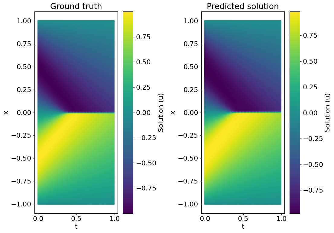
error_u = np.linalg.norm(u_star-u_pred,2)/np.linalg.norm(u_star,2)
print('Error u: %e' %(error_u))
U_pred = griddata(X_star, u_pred.flatten(), (X, T), method='cubic')
Error = 100* np.linalg.norm(Exact - U_pred) / np.linalg.norm(U_pred)
Error u: 6.559859e-02
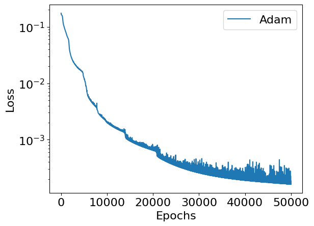
We visulaize the results of our training by plotting the evolution of the loss with respect to the epochs and comparing the predictions by the neural network model with the ground truth.
# plot the results
plt.rcParams.update({'font.size': 16})
print('Loss convergence')
loss = np.array(loss)
range_adam = np.arange(0, Nmax+1)
plt.semilogy(range_adam, loss, label='Adam')
#plt.plot(epochs, loss, label = 'adam optimizer')
#plt.yscale('log')
plt.ylabel('Loss')
plt.xlabel('Epochs')
plt.legend()
plt.show()
Loss convergence
plt.figure(figsize=(16, 8))
plt.subplot(1,3,1)
plt.scatter(X_star[:,1:2], X_star[:,0:1], c = u_star, cmap = 'viridis', s = 5)
plt.colorbar(label='Solution (u)')
plt.xlabel('t')
plt.ylabel('x')
plt.title('Ground truth')

plt.subplot(1,3,2)
plt.scatter(X_star[:,1:2], X_star[:,0:1], c = U_pred, cmap = 'viridis', s = 5)
plt.colorbar(label='Solution (u)')
plt.xlabel('t')
plt.ylabel('x')
plt.title('Predicted solution')

plt.tight_layout()
plt.savefig('Burgers_result.png')
plt.show()