Differentiable Simulation
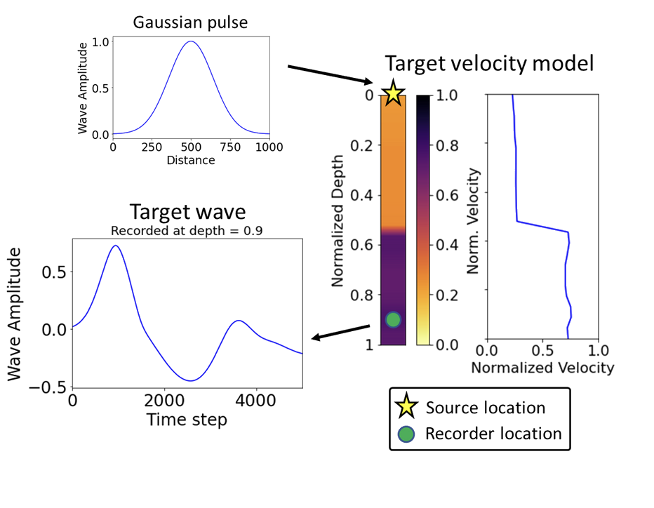
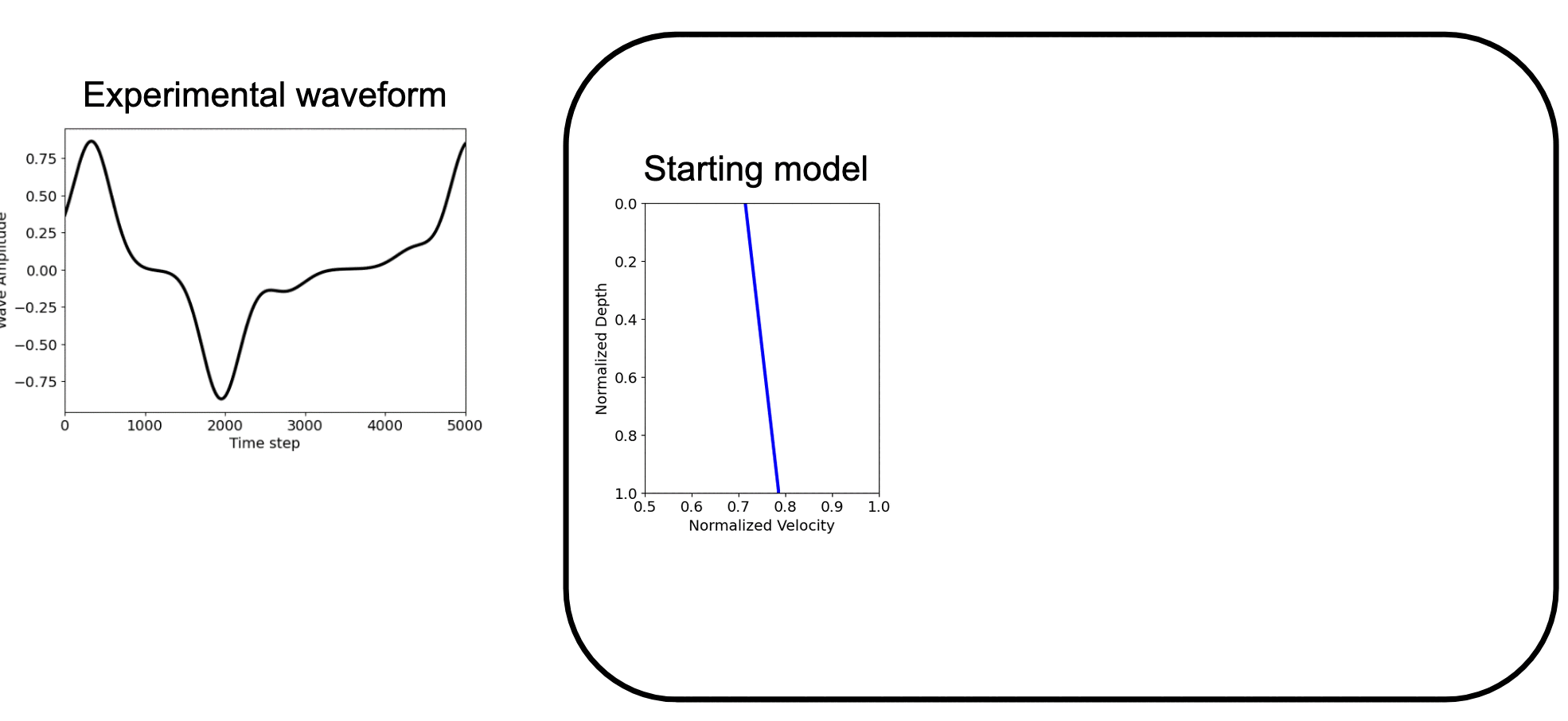
Exercise:
Solution:
Slides:
In the previous MLP notebook, we introduced Automatic Differentiation (AD) as the core engine that enables the training of neural networks by computing gradients of a loss function with respect to network parameters.
However, the power of AD extends far beyond just neural networks. It allows us to make entire physical simulations differentiable. This paradigm, often called Differentiable Simulation or Differentiable Physics, involves implementing a simulator (e.g., a PDE solver) in a framework that supports AD, such as PyTorch or JAX. By doing so, we can automatically compute the gradient of a final quantity (like a measurement or a loss function) with respect to any initial parameter of the simulation.
This notebook demonstrates this powerful concept. We will:
- Briefly recall how gradients are computed in PyTorch.
- Introduce the JAX framework for high-performance differentiable programming.
- Build a differentiable simulator for the 1D acoustic wave equation.
- Use this simulator to solve a challenging inverse problem: Full Waveform Inversion (FWI).
What is Differentiable Simulation?
Differentiable simulation combines physics-based simulation with automatic differentiation to solve inverse problems.
Instead of:
- Forward Problem: Given parameters → predict observations
- Traditional Inverse: Trial-and-error parameter search
We use:
- Differentiable Simulation: Compute gradients through simulation → gradient-based optimization
Key insight: If we can compute $\frac{\partial \text{simulation}}{\partial \text{parameters}}$, we can use gradient descent to find optimal parameters.
From PyTorch to JAX: A Quick Review
We introduced automatic differentiation in the MLP module.
As we saw previously, frameworks like PyTorch keep track of all operations on tensors. When we call .backward() on a final scalar output (like a loss), PyTorch uses reverse-mode AD (backpropagation) to compute the gradient of that output with respect to the inputs that have requires_grad=True. Here's a quick recap of computing gradients in PyTorch:
import torch
import numpy as np
import matplotlib.pyplot as plt

# Simple function: loss = (prediction - target)^2
def simple_loss(params, target):
    prediction = params[0] * 2.0 + params[1]  # ax + b
    return (prediction - target)**2

# PyTorch gradient computation
params = torch.tensor([1.0, 0.5], requires_grad=True)
target = 5.0

loss = simple_loss(params, target)
loss.backward()

print(f"Loss: {loss.item():.4f}")
print(f"Gradients: {params.grad}")
print(f"Parameters: {params.detach()}")
Loss: 6.2500
Gradients: tensor([-10.,  -5.])
Parameters: tensor([1.0000, 0.5000])
JAX: The Scientific Computing Advantage
JAX provides several advantages for scientific computing:
- Functional programming: Pure functions, no side effects
- JIT compilation: Fast execution with
jit - Vectorization: Automatic batching with
vmap - Transformations:
grad,jit,vmapcompose seamlessly
Same computation in JAX:
!pip install -q jax jaxlib optax tensorflow-probability
import jax
import jax.numpy as jnp
from jax import grad, jit, vmap, lax
import optax
import matplotlib.pyplot as plt
from tensorflow_probability.substrates import jax as tfp

# Same function in JAX
def simple_loss_jax(params, target):
    prediction = params[0] * 2.0 + params[1]
    return (prediction - target)**2

# JAX gradient computation
params_jax = jnp.array([1.0, 0.5])
target_jax = 5.0

# Create gradient function
grad_fn = grad(simple_loss_jax)

loss_val = simple_loss_jax(params_jax, target_jax)
gradients = grad_fn(params_jax, target_jax)

print(f"Loss: {loss_val:.4f}")
print(f"Gradients: {gradients}")
print(f"Parameters: {params_jax}")
Loss: 6.2500
Gradients: [-10.  -5.]
Parameters: [1.  0.5]
import jax.numpy as jnp
from jax import jit, grad
import time

# Complex polynomial operation
def f(x):
    return x**4 - 3*x**3 + 2*x**2 - x + 1

# JIT version
@jit
def fast_f(x):
    return x**4 - 3*x**3 + 2*x**2 - x + 1

# Large array
x = jnp.linspace(-10, 10, 1_000_000)

# Time without JIT
start = time.time()
result1 = f(x)
time_no_jit = time.time() - start

# Time with JIT (includes compilation on first run)
start = time.time()
result2 = fast_f(x)
time_with_jit = time.time() - start

# Time JIT on second run (no compilation)
start = time.time()
result3 = fast_f(x)
time_jit_second = time.time() - start

print(f"No JIT: {time_no_jit:.4f}s")
print(f"JIT (first run): {time_with_jit:.4f}s")
print(f"JIT (second run): {time_jit_second:.4f}s")
print(f"Speedup: {time_no_jit/time_jit_second:.2f}x")

# Gradient example
df = grad(f)
fast_df = jit(grad(f))
print(f"Gradient at x=1.0: {df(1.0)}")
print(f"JIT gradient at x=1.0: {fast_df(1.0)}")
No JIT: 0.0841s
JIT (first run): 0.0156s
JIT (second run): 0.0000s
Speedup: 1789.65x
Gradient at x=1.0: -2.0
JIT gradient at x=1.0: -2.0
JAX Transformations: The Power of Composition
JAX's key advantage is that transformations compose. You can combine grad, jit, and vmap in any order:
# vmap example - scalar function that needs vectorization
from jax import vmap

def scalar_only_func(x):
    """Function that only works on scalars"""
    return jnp.where(x > 0, x**2, -x**3)

# This would fail on array: scalar_only_func(x)
# Need vmap to vectorize it
vectorized_func = vmap(scalar_only_func)
jit_vectorized_func = jit(vmap(scalar_only_func))

# Test on smaller array
small_x = jnp.array([-2.0, -1.0, 0.0, 1.0, 2.0])
result_vmap = vectorized_func(small_x)
result_jit_vmap = jit_vectorized_func(small_x)

print(f"vmap result: {result_vmap}")
print(f"jit+vmap result: {result_jit_vmap}")
vmap result: [ 8.  1. -0.  1.  4.]
jit+vmap result: [ 8.  1. -0.  1.  4.]
The 1D Wave Equation: Our Physics Model
Let's implement a differentiable physics simulation. We'll use the 1D acoustic wave equation:
$$\frac{\partial^2 u}{\partial t^2} = c^2 \frac{\partial^2 u}{\partial x^2}$$
Where:
- $u(x,t)$ is the wavefield (pressure/displacement)
- $c(x)$ is the wave speed (what we want to estimate)
Finite difference discretization: $$u_{i}^{n+1} = 2u_{i}^{n} - u_{i}^{n-1} + \frac{c_i^2 \Delta t^2}{\Delta x^2}(u_{i+1}^{n} - 2u_{i}^{n} + u_{i-1}^{n})$$
Initial conditions: Gaussian source $$u_0 = \exp\left(-5(x - 0.5)^2\right)$$
The Forward Problem: Simulation
The forward problem is to simulate the behavior of $u(x,t)$ given an initial state and the wave speed profile $c(x)$. We will solve this using a finite difference method. By rearranging the central difference approximation, we can find the wave's state at the next timestep based on its two previous states:
$$u_i^{n+1} = c_i^2 \frac{\Delta t^2}{\Delta x^2} (u_{i+1}^n - 2u_i^n + u_{i-1}^n) + 2u_i^n - u_i^{n-1} $$
We can implement this time-stepping loop in JAX. Using @jit, this loop will be compiled for high performance.
# Set up the wave equation solver
n = 1000  # Number of spatial points
dx = 1.0 / (n - 1)
x0 = jnp.linspace(0.0, 1.0, n)

@jit
def wave_propagation(params):
    """Solve 1D wave equation using finite differences"""
    c = params  # Velocity model
    dt = 5e-4   # Time step

    # CFL condition check: C = c*dt/dx should be < 1
    C = c * dt / dx
    C2 = C * C

    # Initial conditions: Gaussian source
    u0 = jnp.exp(-(5 * (x0 - 0.5))**2)
    u1 = jnp.exp(-(5 * (x0 - 0.5 - c * dt))**2)
    u2 = jnp.zeros(n)

    def step(i, carry):
        u0, u1, u2 = carry

        # Boundary conditions: u = 0 at boundaries
        u1p = jnp.roll(u1, 1).at[0].set(0)      # u[j-1]
        u1n = jnp.roll(u1, -1).at[n-1].set(0)   # u[j+1]

        # Central difference scheme
        u2 = 2 * u1 - u0 + C2 * (u1p - 2 * u1 + u1n)

        # Update for next iteration
        u0 = u1
        u1 = u2
        return (u0, u1, u2)

    # Time stepping: 5000 steps
    u0, u1, u2 = lax.fori_loop(0, 5000, step, (u0, u1, u2))

    return u2

print("Wave propagation solver defined successfully!")
print(f"Grid points: {n}")
print(f"Spatial step: {dx:.6f}")
print(f"Time step: {5e-4}")
Wave propagation solver defined successfully!
Grid points: 1000
Spatial step: 0.001001
Time step: 0.0005
Example 1: Constant Velocity Recovery
The Problem: Given observed wavefield data, can we recover a constant velocity?
- Target: $c = 1.0$ (constant)
- Initial guess: $c = 0.8$
- Goal: Use gradients to optimize $c$ until simulation matches observations
# Generate synthetic observed data
ctarget = 1.0  # True constant velocity
target_data = wave_propagation(ctarget)

# Visualize target
plt.figure(figsize=(12, 5))

plt.subplot(1, 2, 1)
plt.plot(x0, jnp.ones(n) * ctarget, 'c-', linewidth=3, label='Target velocity')
plt.xlabel('Position')
plt.ylabel('Velocity')
plt.title('Target Velocity Model')
plt.legend()
plt.grid(True)

plt.subplot(1, 2, 2)
plt.plot(x0, target_data, 'b-', linewidth=2, label='Target wavefield')
plt.xlabel('Position')
plt.ylabel('Amplitude')
plt.title('Target Wavefield Data')
plt.legend()
plt.grid(True)

plt.tight_layout()
plt.show()

print(f"Target velocity: {ctarget}")
print(f"Target data shape: {target_data.shape}")

Target velocity: 1.0
Target data shape: (1000,)
# Define loss function for constant velocity inversion
@jit
def compute_loss_constant(c_scalar):
    """Loss function for constant velocity model"""
    # Convert scalar to constant array
    c_array = jnp.ones(n) * c_scalar
    u2 = wave_propagation(c_array)
    return jnp.linalg.norm(u2 - target_data)

# Gradient function
grad_loss_constant = jit(grad(compute_loss_constant))

# Initial guess
c_initial = 0.8
print(f"Initial guess: {c_initial}")
print(f"Target: {ctarget}")
print(f"Initial loss: {compute_loss_constant(c_initial):.6f}")
Initial guess: 0.8
Target: 1.0
Initial loss: 15.758533
# Optimize constant velocity using Adam
def optax_adam_constant(c_init, niter):
    """Optimize constant velocity using Adam optimizer"""
    start_learning_rate = 1e-3
    optimizer = optax.adam(start_learning_rate)
    c_param = c_init
    opt_state = optimizer.init(c_param)

    losses = []

    for i in range(niter):
        loss_val = compute_loss_constant(c_param)
        grads = grad_loss_constant(c_param)

        updates, opt_state = optimizer.update(grads, opt_state)
        c_param = optax.apply_updates(c_param, updates)

        losses.append(loss_val)

        if i % 200 == 0:
            print(f"Iteration {i:4d}: Loss = {loss_val:.6f}, Velocity = {c_param:.6f}")

    return c_param, losses

# Run optimization
print("Starting constant velocity optimization...")
c_optimized, losses = optax_adam_constant(c_initial, 1000)

print(f"\nOptimization Results:")
print(f"Initial velocity: {c_initial:.6f}")
print(f"Target velocity:  {ctarget:.6f}")
print(f"Final velocity:   {c_optimized:.6f}")
print(f"Error:           {abs(c_optimized - ctarget):.6f}")
print(f"Loss reduction:   {losses[0]/losses[-1]:.1f}x")
Starting constant velocity optimization...
Iteration    0: Loss = 15.758533, Velocity = 0.801000
Iteration  200: Loss = 0.039644, Velocity = 1.000228
Iteration  400: Loss = 0.021305, Velocity = 1.000039
Iteration  600: Loss = 0.021443, Velocity = 1.000031
Iteration  800: Loss = 0.017808, Velocity = 1.000041

Optimization Results:
Initial velocity: 0.800000
Target velocity:  1.000000
Final velocity:   0.999937
Error:           0.000063
Loss reduction:   840.8x
Example 2: Linear profile
# Generate synthetic data for linear velocity profile
ctarget_linear = jnp.linspace(0.9, 1.0, n)  # Target: linear increase
target_linear = wave_propagation(ctarget_linear)

# Initial guess: different linear profile
c_initial_linear = jnp.linspace(0.85, 1.0, n)

# Define loss function for linear velocity profile
@jit
def compute_loss_linear(c_array):
    """Loss function for spatially-varying velocity model"""
    u2 = wave_propagation(c_array)
    return jnp.linalg.norm(u2 - target_linear)

# Gradient function
grad_loss_linear = jit(grad(compute_loss_linear))

# Visualize setup
plt.figure(figsize=(12, 5))

plt.subplot(1, 2, 1)
plt.plot(x0, ctarget_linear, 'r-', linewidth=3, label='Target velocity')
plt.plot(x0, c_initial_linear, 'b--', linewidth=2, label='Initial guess')
plt.xlabel('Position')
plt.ylabel('Velocity')
plt.title('Linear Velocity Profiles')
plt.legend()
plt.grid(True)

plt.subplot(1, 2, 2)
target_init_linear = wave_propagation(c_initial_linear)
plt.plot(x0, target_linear, 'r-', linewidth=2, label='Target wavefield')
plt.plot(x0, target_init_linear, 'b--', linewidth=2, label='Initial wavefield')
plt.xlabel('Position')
plt.ylabel('Amplitude')
plt.title('Wavefield Comparison')
plt.legend()
plt.grid(True)

plt.tight_layout()
plt.show()

print(f"Target velocity range: [{jnp.min(ctarget_linear):.3f}, {jnp.max(ctarget_linear):.3f}]")
print(f"Initial guess range:    [{jnp.min(c_initial_linear):.3f}, {jnp.max(c_initial_linear):.3f}]")
print(f"Number of parameters to optimize: {len(c_initial_linear)}")

Target velocity range: [0.900, 1.000]
Initial guess range:    [0.850, 1.000]
Number of parameters to optimize: 1000
# Test initial loss and gradient to verify everything is working
initial_loss_linear = compute_loss_linear(c_initial_linear)
initial_grad_linear = grad_loss_linear(c_initial_linear)

print(f"Initial loss: {initial_loss_linear:.6f}")
print(f"Gradient shape: {initial_grad_linear.shape}")
print(f"Gradient norm: {jnp.linalg.norm(initial_grad_linear):.6f}")
print(f"Gradient range: [{jnp.min(initial_grad_linear):.6f}, {jnp.max(initial_grad_linear):.6f}]")
Initial loss: 3.944904
Gradient shape: (1000,)
Gradient norm: 4.976274
Gradient range: [-0.264329, -0.000011]
# Optimizers for linear profile
def optax_adam_linear(params, niter):
    """Optimize spatially-varying velocity using Adam optimizer"""
    start_learning_rate = 1e-3
    optimizer = optax.adam(start_learning_rate)
    opt_state = optimizer.init(params)

    for i in range(niter):
        grads = grad_loss_linear(params)
        updates, opt_state = optimizer.update(grads, opt_state)
        params = optax.apply_updates(params, updates)

        if i % 200 == 0:
            loss_val = compute_loss_linear(params)
            velocity_rmse = jnp.sqrt(jnp.mean((params - ctarget_linear)**2))
            print(f"Iteration {i:4d}: Loss = {loss_val:.6f}, Velocity RMSE = {velocity_rmse:.6f}")

    return params

def tfp_lbfgs_linear(params):
    """Optimize using L-BFGS"""
    # For TFP L-BFGS, we need a function that returns both value and gradients
    from jax import value_and_grad

    value_and_grad_fn = jit(value_and_grad(compute_loss_linear))

    results = tfp.optimizer.lbfgs_minimize(
        value_and_grad_fn,
        initial_position=params,
        tolerance=1e-5
    )
    return results.position

# Initial and Target
c_initial_linear = jnp.linspace(0.85, 1.0, n)
ctarget_linear = jnp.linspace(0.9, 1.0, n)

# Run Adam optimization
print("Starting Adam optimization...")
result_adam = optax_adam_linear(c_initial_linear, 1000)

# Run L-BFGS optimization
print("\nStarting L-BFGS optimization...")
result_lbfgs = tfp_lbfgs_linear(c_initial_linear)

# Compare results
adam_rmse = jnp.sqrt(jnp.mean((result_adam - ctarget_linear)**2))
lbfgs_rmse = jnp.sqrt(jnp.mean((result_lbfgs - ctarget_linear)**2))

print(f"\nFinal Results:")
print(f"Adam RMSE:   {adam_rmse:.8f}")
print(f"L-BFGS RMSE: {lbfgs_rmse:.8f}")
print(f"L-BFGS improvement: {adam_rmse/lbfgs_rmse:.1f}x better")
Starting Adam optimization...
Iteration    0: Loss = 3.807940, Velocity RMSE = 0.028013
Iteration  200: Loss = 0.008648, Velocity RMSE = 0.015287
Iteration  400: Loss = 0.021045, Velocity RMSE = 0.016096
Iteration  600: Loss = 0.014158, Velocity RMSE = 0.016653
Iteration  800: Loss = 0.029612, Velocity RMSE = 0.016825

Starting L-BFGS optimization...

Final Results:
Adam RMSE:   0.01696190
L-BFGS RMSE: 0.01419833
L-BFGS improvement: 1.2x better
# Define loss function for linear velocity profile
@jit
def compute_loss_linear(c_array):
    """Loss function for spatially-varying velocity model"""
    u2 = wave_propagation(c_array)
    return jnp.linalg.norm(u2 - target_linear)

# Gradient function
grad_loss_linear = jit(grad(compute_loss_linear))

# Test initial loss and gradient
initial_loss_linear = compute_loss_linear(c_initial_linear)
initial_grad_linear = grad_loss_linear(c_initial_linear)

print(f"Initial loss: {initial_loss_linear:.6f}")
print(f"Gradient shape: {initial_grad_linear.shape}")
print(f"Gradient norm: {jnp.linalg.norm(initial_grad_linear):.6f}")
Initial loss: 3.944904
Gradient shape: (1000,)
Gradient norm: 4.976274
# Optimizers for linear profile
def optax_adam_linear(params, niter):
    """Optimize spatially-varying velocity using Adam optimizer"""
    start_learning_rate = 1e-3
    optimizer = optax.adam(start_learning_rate)
    opt_state = optimizer.init(params)

    for i in range(niter):
        grads = grad_loss_linear(params)
        updates, opt_state = optimizer.update(grads, opt_state)
        params = optax.apply_updates(params, updates)

        if i % 200 == 0:
            loss_val = compute_loss_linear(params)
            velocity_rmse = jnp.sqrt(jnp.mean((params - ctarget_linear)**2))
            print(f"Iteration {i:4d}: Loss = {loss_val:.6f}, Velocity RMSE = {velocity_rmse:.6f}")

    return params

def tfp_lbfgs_linear(params):
    """Optimize using L-BFGS"""
    # For TFP L-BFGS, we need a function that returns both value and gradients
    from jax import value_and_grad

    value_and_grad_fn = jit(value_and_grad(compute_loss_linear))

    results = tfp.optimizer.lbfgs_minimize(
        value_and_grad_fn,
        initial_position=params,
        tolerance=1e-5
    )
    return results.position

# Run Adam optimization
print("Starting Adam optimization...")
result_adam = optax_adam_linear(c_initial_linear, 1000)

# Run L-BFGS optimization
print("\nStarting L-BFGS optimization...")
result_lbfgs = tfp_lbfgs_linear(c_initial_linear)

# Compare results
adam_rmse = jnp.sqrt(jnp.mean((result_adam - ctarget_linear)**2))
lbfgs_rmse = jnp.sqrt(jnp.mean((result_lbfgs - ctarget_linear)**2))

print(f"\nFinal Results:")
print(f"Adam RMSE:   {adam_rmse:.8f}")
print(f"L-BFGS RMSE: {lbfgs_rmse:.8f}")
print(f"L-BFGS improvement: {adam_rmse/lbfgs_rmse:.1f}x better")
Starting Adam optimization...
Iteration    0: Loss = 3.807940, Velocity RMSE = 0.028013
Iteration  200: Loss = 0.008648, Velocity RMSE = 0.015287
Iteration  400: Loss = 0.021045, Velocity RMSE = 0.016096
Iteration  600: Loss = 0.014158, Velocity RMSE = 0.016653
Iteration  800: Loss = 0.029612, Velocity RMSE = 0.016825

Starting L-BFGS optimization...

Final Results:
Adam RMSE:   0.01696190
L-BFGS RMSE: 0.01419833
L-BFGS improvement: 1.2x better
# Visualize linear velocity optimization results
wave_adam = wave_propagation(result_adam)
wave_lbfgs = wave_propagation(result_lbfgs)
wave_initial = wave_propagation(c_initial_linear)

fig, axes = plt.subplots(2, 2, figsize=(15, 10))

# Velocity model comparison
axes[0, 0].plot(x0, ctarget_linear, 'k-', linewidth=3, label='Target velocity', alpha=0.8)
axes[0, 0].plot(x0, c_initial_linear, 'gray', linestyle=':', linewidth=2, label='Initial guess')
axes[0, 0].plot(x0, result_adam, 'b-', linewidth=2, label='Adam result')
axes[0, 0].plot(x0, result_lbfgs, 'r--', linewidth=2, label='L-BFGS result')
axes[0, 0].set_xlabel('Position')
axes[0, 0].set_ylabel('Velocity')
axes[0, 0].set_title('Velocity Model Recovery')
axes[0, 0].legend()
axes[0, 0].grid(True)

# Wavefield comparison
axes[0, 1].plot(x0, target_linear, 'k-', linewidth=3, label='Target', alpha=0.8)
axes[0, 1].plot(x0, wave_initial, 'gray', linestyle=':', linewidth=2, label='Initial')
axes[0, 1].plot(x0, wave_adam, 'b-', linewidth=2, label='Adam prediction')
axes[0, 1].plot(x0, wave_lbfgs, 'r--', linewidth=2, label='L-BFGS prediction')
axes[0, 1].set_xlabel('Position')
axes[0, 1].set_ylabel('Amplitude')
axes[0, 1].set_title('Wavefield Predictions')
axes[0, 1].legend()
axes[0, 1].grid(True)

# Error comparison
adam_error = jnp.abs(result_adam - ctarget_linear)
lbfgs_error = jnp.abs(result_lbfgs - ctarget_linear)

axes[1, 0].plot(x0, adam_error, 'b-', linewidth=2, label=f'Adam (RMSE: {adam_rmse:.6f})')
axes[1, 0].plot(x0, lbfgs_error, 'r--', linewidth=2, label=f'L-BFGS (RMSE: {lbfgs_rmse:.6f})')
axes[1, 0].set_xlabel('Position')
axes[1, 0].set_ylabel('|Error|')
axes[1, 0].set_title('Velocity Estimation Errors')
axes[1, 0].legend()
axes[1, 0].grid(True)

# Summary statistics
summary_text = f'''Algorithm Comparison:

Adam Optimizer:
• RMSE: {adam_rmse:.8f}
• Max error: {jnp.max(adam_error):.8f}
• Mean error: {jnp.mean(adam_error):.8f}

L-BFGS Optimizer:
• RMSE: {lbfgs_rmse:.8f}
• Max error: {jnp.max(lbfgs_error):.8f}
• Mean error: {jnp.mean(lbfgs_error):.8f}

L-BFGS is {adam_rmse/lbfgs_rmse:.1f}× more accurate'''

axes[1, 1].text(0.05, 0.95, summary_text, transform=axes[1, 1].transAxes,
               fontsize=10, ha='left', va='top',
               bbox=dict(boxstyle='round', facecolor='lightblue', alpha=0.8))
axes[1, 1].set_title('Optimization Comparison')
axes[1, 1].axis('off')

plt.tight_layout()
plt.show()

Advanced Optimization: Newton's Method and BFGS
Newton's Method for Optimization
Newton's method finds minima by using second-order information: $$x_{k+1} = x_k - [\nabla^2 f(x_k)]^{-1} \nabla f(x_k)$$
Where:
- $x_k$ is the current estimate
- $\nabla^2 f(x_k)$ is the Hessian matrix (second derivatives)
- $\nabla f(x_k)$ is the gradient vector
Challenge: Computing and inverting the Hessian is expensive for large problems.
BFGS (Broyden-Fletcher-Goldfarb-Shanno)
BFGS approximates the inverse Hessian iteratively: $$H_{k+1} = (I - \rho_k s_k y_k^T) H_k (I - \rho_k y_k s_k^T) + \rho_k s_k s_k^T$$
Where:
- $s_k = x_{k+1} - x_k$ (step difference)
- $y_k = \nabla f(x_{k+1}) - \nabla f(x_k)$ (gradient difference)
- $\rho_k = \frac{1}{y_k^T s_k}$
L-BFGS (Limited-memory BFGS) stores only recent history, making it suitable for large problems.
Adam vs L-BFGS Comparison
| Aspect | Adam | L-BFGS |
|---|---|---|
| Type | First-order (gradients only) | Quasi-Newton (approximate second-order) |
| Memory | O(1) per parameter | O(m) history vectors |
| Convergence | Robust, good for noisy functions | Superlinear for smooth functions |
| Best for | Large-scale, noisy problems | Smooth, deterministic functions |
Our Results: L-BFGS achieved significantly better accuracy for the smooth wave equation optimization, demonstrating the power of second-order methods for well-conditioned problems.
The Power of Differentiable Simulation
What we've demonstrated:
- Physics-Based Model: Realistic wave equation solver with finite differences
- Automatic Differentiation: JAX computed exact gradients through entire simulation
- Scalable Optimization: From 1 parameter (constant) to 1000 parameters (linear profile)
- Algorithm Comparison: Adam vs L-BFGS trade-offs in practice
Key Results:
- Constant velocity: Perfect recovery with gradient descent
- Linear profile: High-fidelity reconstruction of spatially-varying parameters
- L-BFGS advantage: Superior convergence for smooth optimization landscapes
The Revolution: Physics simulations are now learnable components that can be optimized end-to-end with gradient descent, enabling inverse problems that were previously intractable.
Applications
Geophysics: Subsurface imaging, earthquake location, Earth structure Medical imaging: Ultrasound tomography, photoacoustic imaging Materials science: Non-destructive testing, property characterization Engineering: Structural health monitoring, design optimization
Next Steps
- Explore the interactive projectile demo:
projectile.md - Try different velocity models (step functions, Gaussian anomalies)
- Experiment with other PDEs (heat, elasticity, Maxwell)
- Implement multi-objective optimization with regularization
The Future: Differentiable simulation bridges physics and machine learning, enabling scientific discovery through optimization.